Loan Pricing¶

Pricing of a loan, just like any other product, is influenced by both the cost to produce and the market.

And so there are two methods to deriving an interest rate for a loan:

Capital-Driven:
- what interest rate is required to justify the allocation of capital?
Market-Driven:
- what rate is implied in the market?
- derived from various market-related exposures

The two methods are not exclusive. Fico should consider both approaches when loan pricing as circumstances may reveal information:

$\text{Market-Driven Rate} >>> \text{Capital Driven Rate}$

Fico either has some competitive advantage or it is underpricing risk

$\text{Capital Driven Rate} >>> \text{Market-Driven Rate}$

Fico has a competitive disadvantage or it is overpricing risk

Capital Driven¶

Loan income is compared to a hurdle rate, which can be set as the Weighted Average Cost of Capital (WACC) for the company/investor/project.

\[\text{WACC} = r_{tgt} = w_{debt}*r_{debt} + w_{equity}*r_{equity}\]

$\qquad\qquad\qquad\qquad\qquad\textit{where:}$

\[\begin{split}\\w_{debt} = \frac{D}{D+E}\end{split}\]

$\qquad$or simply as the cost of equity, to take the investor perspective:

\[r_{tgt} = r_{equity}\]

$\qquad$ The hurdle rate may also be set relative to other investment opportunities (and thereby seen as an opportunity cost).

The interest rate required for an individual loan to meet the hurdle rate is:

\[\begin{split}\begin{alignat*}{0} \qquad\text{int}_i = \frac{r_{tgt}*(D_i+E_i) + exp_i}{EAD_i} \\\textit{where:} \\\qquad exp_i = \text{expected losses + non-recovery related expenses like salaries, taxes, etc.} \\\qquad D_i, E_i = \text{debt and equity contribution required for the individual loan} \\\qquad D_i + E_i = EAD_i \end{alignat*}\end{split}\]

Equity Only

We will estimate pricing for loans where Fico is funded entirely by equity.

Assume:

$r_{tgt} = .12$
$exp_i = EL_i$ i.e. Fico has no expenses save for loan losses
Supported entirely by equity capital

For this exercise, we created a new portfolio via the approach in loss models with the following properties:

Number of Loans: 20
Total Outstanding: $2,000,000
Expected Loss: $21,076.89
Required Equity (99.95% VaR): $281,538.97

With that portfolio distribution, we now want to consider how to price 3 loans in the portfolio. The loans have details as follows:

[13]:

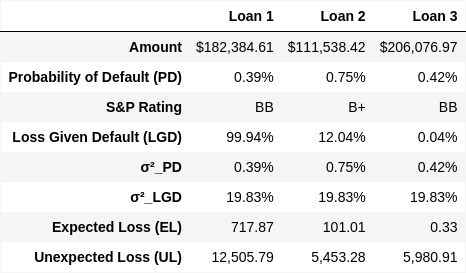
We can do quick math on each loan to find the interest rate required to meet hurdle:

[14]:

def calc_ret(rev, exp, cap):
    return (rev - exp) / cap

def int_to_make_hurdle(exp, loan, equity, hurdle):
    return (hurdle*equity + exp) / loan

hurdle = .12
exp = el

debt = 0
equity = loan_ead
req_int = int_to_make_hurdle(exp, loan_ead, equity, hurdle)

[15]:

Unsurprisingly, even the lowest risk loan requires at least 12% interest rate. This is way above market for these types of loans.

Leverage can be utilized to lower the hurdle rate.

Mix of Debt and Equity

To show how we can incorporate leverage, we modify our assumptions. For each loan, we will assume that we only need to hold the UL for each loan as equity. The rest of Fico’s capital will be debt, borrowed at 3%.

Assume:

$r_{tgt} = .12$
$E_i = UL_i$
$D_i = EAD_i - E_i$
$exp_i = EL_i + D_i*r_{debt}$
$r_{debt} = .03$

[16]:

equity = ul
debt = loan_ead - equity

cost_of_debt = .03
int_on_debt = debt * cost_of_debt
exp = el + int_on_debt

req_int = int_to_make_hurdle(exp, loan_ead, equity, hurdle)

[18]:

df_loan_metrics_w_leverage.style.format({
    'Amount': '{:,.2f}',
    'Probability of Default (PD)': '{:.2%}',
    'Loss Given Default (LGD)': '{:.2%}',
    'Expected Loss (EL)': '{:,.2f}',
    'Required Interest Rate': '{:.2%}'
})

[18]:

	Amount	Probability of Default (PD)	Loss Given Default (LGD)	Expected Loss (EL)	Required Interest Rate
Loan 1	182,384.61	0.39%	99.94%	717.87	4.01%
Loan 2	111,538.42	0.75%	12.04%	101.01	3.53%
Loan 3	206,076.97	0.42%	0.04%	0.33	3.26%

[19]:

await dfi.export_async(df_loan_metrics_w_leverage.style.format({
    'Amount': '{:,.2f}',
    'Probability of Default (PD)': '{:.2%}',
    'Loss Given Default (LGD)': '{:.2%}',
    'Expected Loss (EL)': '{:,.2f}',
    'Required Interest Rate': '{:.2%}'
}), '_static/pricing_3_loan_metrics_table_w_leverage.png')

Image(filename='_static/pricing_3_loan_metrics_table_w_leverage.png')

[19]:

We can see how the mix of debt and equity has helped to improve loan pricing, which should make Fico more competitive in the market place.

Market Driven¶

Interest rates charged on government bonds, corporate debt, or any other loan are generally understood to be derived from the following components:

Real risk-free rate
- generalyl understood to be a function of the “inherent” time value of money, which requires an incentive to delay consumption.
- I actually believe it has more to do with increasing real consumption; my working theory is the real risk-free is the value-add created by increasing consumption.
Inflation premium
Liquidity premium
- understood as relative cost to sell the debt
- smaller amounts, poorer credit risks, less desirable jurisdictions, lower coupons
Credit Risk premium
Margin
- in an efficient bond market, pricing theory dictates that there would be not “profit” to the holder (or the issuer).
- but as a service provider, margin can be incorporated

These factors are observable, although every borrower / loan has its unique qualities that will alter the components slightly from observable values.

So all-in rate derived as:

\[r + r_{inf} + r_{lqd} + r_{cred} + r_{prof}\]

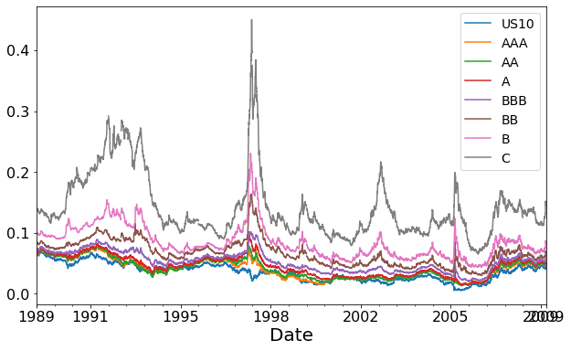
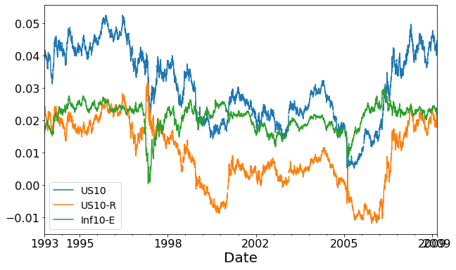
We can infer the components from available market data, such as this chart of corporate bond yields.

[20]:

yields = get_yields()
ax = yields.plot(figsize=(10,6))

ax.xaxis.set_major_formatter(DateFormatter('%Y'))
ax.tick_params('x', labelrotation=0)

for label in ax.get_xticklabels():
    label.set_horizontalalignment('center')

plt.show()

[21]:

infsers = ['DGS10', 'DFII10', 'T10YIE']
frames = [framer(ser) for ser in infsers]

infs = frames[0]
for f in frames[1:]:
    infs = infs.merge(f, on='Date')
infs = infs.set_index('Date')

infs = infs.apply(numeric_coerce)
infs.columns = ['US10', 'US10-R', 'Inf10-E']
infs /= 100

[22]:

ax = infs.plot(figsize=(10,6))

ax.xaxis.set_major_formatter(DateFormatter('%Y'))
ax.tick_params('x', labelrotation=0)

for label in ax.get_xticklabels():
    label.set_horizontalalignment('center')

plt.show()

[23]:

us, real, inf = infs.iloc[-1].to_list()

$r + r_{inf}$ = 2.11% + 2.23% = 4.34%

US 10 Year = 4.34%

[25]:

aaa = yields.AAA.iloc[-1]
lqd = aaa - us

AAA Corp = 4.78%

$r_{lqd} = r_{aaa} - r - r_{inf}$ = 4.78% 2.11% - 2.23% = 0.44%

[27]:

bbb = yields.BBB.iloc[-1]
cred = bbb - aaa

BBB Corp = 5.60%

$r_{cred} = r_{bbb} - r - r_{inf} - r_{lqd}$ = 5.60% - 2.11% - 2.23% - 0.44%= 0.82%

$r + r_{inf} + r_{lqd} + r_{cred}$

= 2.11% + 2.23% + 0.44% + 0.82%

= 5.60%