Credit Risk Modelling
In this section, we will build the loss model for the HTS Customer Finance Program.
Why Should Fico Care About Predicting Losses?
1. Equity
How much equity does Fico need to absorb potential lossess?
Fico expects to have average losses of
xper year, but in any one year, Fico might experience losses10xor100x.Fico needs an equity base to support those extreme years.
2. Pricing
Loan losses are Fico’s largest expense.
Interest rate to charge borrower is a function of how much we expect to lose.
3. Return
Is this loan worthwhile?
Is this entire loan portfolio worthwhile?
The 3 Components of Loss:
Exposure at Default, EAD: amount that is owed at the time the borrower defaults (principal only)
Probability of Default, PD: the likelihood a borrower will not repay the loan
Loss Given Default, LGD: the actual amount of loss on the loan, if the borrower defaults.
The expected average loss on a loan portfolio in a given year is a very simple formula:
Loss Distribution
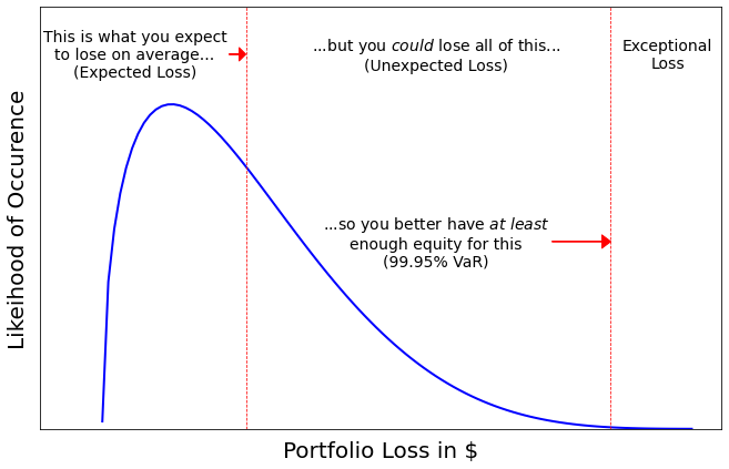
To predict losses, we need to map our portfolio onto a Loss Distribution.
The parameters of the distribution are unique to each loan book at any moment in time based on:
number of loans
size of loans
ratings of different borrowers
value of assets under each loan
correlation of defaults and correlation of defaults / asset values
Here are some key terms we will use:
Beta Distribution
the distribution of losses in any given year is generally believed to follow a Beta distribution, where very small losses occur the vast majority of years and very large losses occur sporadically.
Expected Loss (EL)
the mean value of the Loss distribution
if the loan book is correctly modelled, i.e. borrower PDs are accurate, equipment market values are accurate etc., this is the average amount of losses Fico should experience in the long-term.
Unexpected Loss (UL)
one standard deviation from the mean of the Loss distribution
varies by loan book but typically loan losses should be less than UL in 80% of years
Economic Capital (EC)
amount of equity required to absorb extreme events
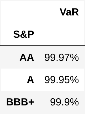
sometimes set using Value-at-Risk (VaR)
agencies typically consider VaR as a factor for determining a bank’s credit rating
a 99.95% VaR can be interpreted as “this level of losses is expected in 5 out of every 10,000 years”
[40]:
Other Considerations
Correlation of Defaults:
exogeneous factors may result in borrowers defaulting at the same time and more than they would independently. This increases losses at those times.
Correlation of PD and LGD:
simplest (and prevailing) assumption is PD and LGD are uncorrelated
more realistic assumption is PD and LGD are correlated
3rd party providers
data and modelling tools can be purchased from 3rd parties
Examples:
Process to Determine Loss Distribution
Determine PD, LGD, LGD distribution, PD correlations, PD/LGD correlations (if any).
Find EL and UL.
Run Monte Carlo simulations. Determine the Loss Distribution of the portfolio.
Find best fit for beta distribution
Find Economic Capital through VaR (for whatever credit rating desired).
Fico needs equity equal to at least the Economic Capital.
Extreme Value Theory can be used to protect against even greater tail risks.
Probability of Default
determined through analysis of company financial statements, business/industry risks, and exogenous factors like economic activity.
bond/credit ratings are categorized based on PD. The S&P ratings and their analogous PDs are shown below:

credit ratings BBB+ and greater are typically considered investment grade.
rating BBB to CCC+/CCC are consider “junk” or speculative.
CCC+/CCC or worse is typically considered a default
The distribution of ratings within a portfolio are often unique to the portfolio: what borrowers are targeted? what is risk management quality? etc.
For now, it is useful to assume a portfolio with normally distributed PDs with the following parameters:
\(\mu = .44\)%
\(\sigma = .2\)%
The portfolio has a PD distribution as per below. Note the x-axis increases exponentially, so the normal distribution is skewed.
[42]:
import warnings

with warnings.catch_warnings():
    warnings.filterwarnings("ignore")

    mu = .0044
    std = .002

    x = np.linspace(0,1,10000)
    y = norm.pdf(x, mu, std)

    fig, ax = plt.subplots(figsize=(10,6))
    ax.plot(x, y, 'k-', lw=2)

    ax.set_xscale('log')

    ratlabs = ['', '', 'AAA', 'A-', 'B+', 'CCC+', 'D', '']
    ax.set_xticklabels([f'{val:.2%}\n{ratlab}' for val, ratlab in zip(ax.get_xticks(), ratlabs)])

    plt.suptitle('Portfolio Distribution of PD')

    plt.show()
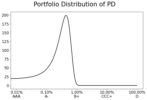
The portfolio, on average, would have “junk” exposure, but we can see above that the majority of borrowers would be rated stronger.
Loss Given Default
A detailed discussion of LGD is here. For this exercise, we are just looking for a credible way to model it.
often modelled based on the Beta distribution, as per Moody’s LossCalc
the Beta distribution isn’t great for leases, because it does not allow for recovery gains. More complex models should be considered for leasing.
There is limited data available on equipment recoveries, but one study shows recoveries in various European countries between 1976 and 2002. The average LGD and standard deviation varied quite widely, so judging by the wind we’ll go with:
the Beta distribution is generally parameterized as follows:
but it can also be built from the mean and standard deviation:
We have some helper functions written derive \(\alpha\)/\(\beta\) from \(\mu\)/\(\sigma\).
[43]:
mu = .4
std = .4

a, b = beta_params_from_descript(mu, std**2)
This results in alpha = 0.2 and beta = 0.3. Plug those into Beta(0.2, 0.3) and you get the following LGD distribution:
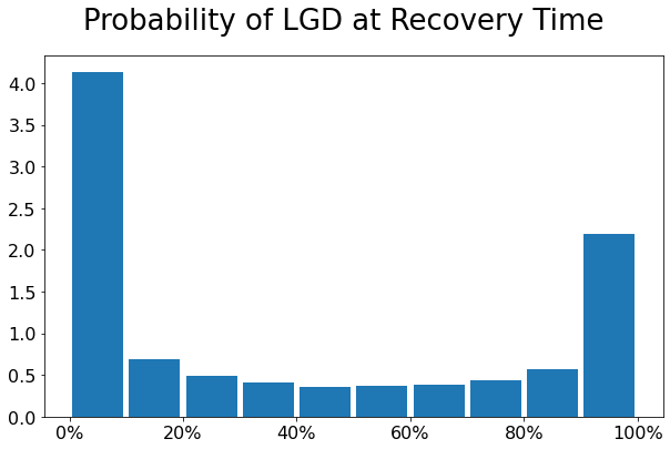
We can see that the majority of defaults result in almost no loss or an entire loss.
Loss Models
A loss model must:
determine expected losses at loan level
determine expected losses at portfolio level, and how to aggregrate based on correlated outcomes.
Loss models have developed increasing complexity in the past two decades but regulatory requirements of banks and other FIs still center around Basel 2, which has a basic assumption that PD and LGD are uncorrelated. This assumption has been questioned more recently (and intuitively seems weak).
We will show examples for both (though the latter is much more complicated and so the example is partial).
Model 1: PD / LGD Uncorrelated
Assumes that the loss given default on the loan is not related to the default. Picture an asset whose value does not change regardless of economic circumstances.
The model does account for correlation of default among obligors. i.e. there is some exogneous factor(s) that cause bororwers to default at the same time. This makes sense intuitively.
Single Loan
often shown for each dollar of EAD as:
\begin{equation} UL = EAD * \sqrt(PD*\sigma^2_{LGD} + LGD^2*\sigma^2_{PD}) \\\sigma^2_{PD} = (PD)(1-PD) \\\sigma^2_{LGD} = \frac{\alpha\beta}{(\alpha+\beta)^2(\alpha+\beta+1)} \end{equation}
Multiple Loans
\begin{equation} EL_p = \sum^n_{i=1}{EAD_i*PD_i*LGD_i} \\UL_p = \sqrt{\sum_i\sum_j\rho_{ij}w_iw_jUL_iUL_j} \end{equation}
where:
\begin{equation} p_{i,j} = 1 \text{ if }i=j \\w_i = EAD_i / EAD_p \\EAD_p = \sum^n_{i=0}EAD_i \\UL_i = EAD_i * \sqrt(PD^2_i*\sigma^2_{LGD, i} + LGD^2_i*\sigma^2_{PD,i}) \end{equation}
Example
Assumptions:
5 loans
$500K total outstanding
PD is Bernoulli variable, however, generated randomly via Normal distribution as per above.
LGD is Beta variable as per above
all loans are for the same asset, therefore, have same LGD distribution
PD and LGD are uncorrelated
First, we create the loan exposures.
[47]:
# Loan Portfolio
n = 5
loans_t = 5*10**5
randloans = np.random.uniform(0.1,1,n)
EAD = (randloans / randloans.sum())*loans_t
w = EAD / EAD.sum()
print (f'Confirming Portfolio Size: {EAD.sum():,.2f}')
Confirming Portfolio Size: 500,000.00
Now, we created the PDs for each loan.
[48]:
# PD for each borrower/loan.
pd_mu = 0.0044
pd_std = 0.002
p_of_d = np.random.normal(pd_mu, pd_std, n)
count, bins = np.histogram(p_of_d, bins=PDs)
binned = np.digitize(p_of_d, bins)
rats = np.array(SPs)[binned]

p_of_d = np.where(p_of_d<0, 0, p_of_d)

pd_var = bern.var(p_of_d)     # PD for each individual loan is bernoulli distributed and has its own variance.
And the LGDs for each loan.
[49]:
# LGD
lgd_mu = .4
lgd_std = .4

a, b = beta_params_from_descript(lgd_mu, lgd_std**2)
lgd_freeze = beta(a, b)
lgd = lgd_freeze.rvs(size=n)

lgd_var = np.repeat(lgd.var(), n)
Then EL and UL can be calculated as:
[50]:
el = EAD*p_of_d*lgd
ul = loan_ul(EAD, p_of_d, lgd, pd_var, lgd_var)
We show the results for each individual loan below:
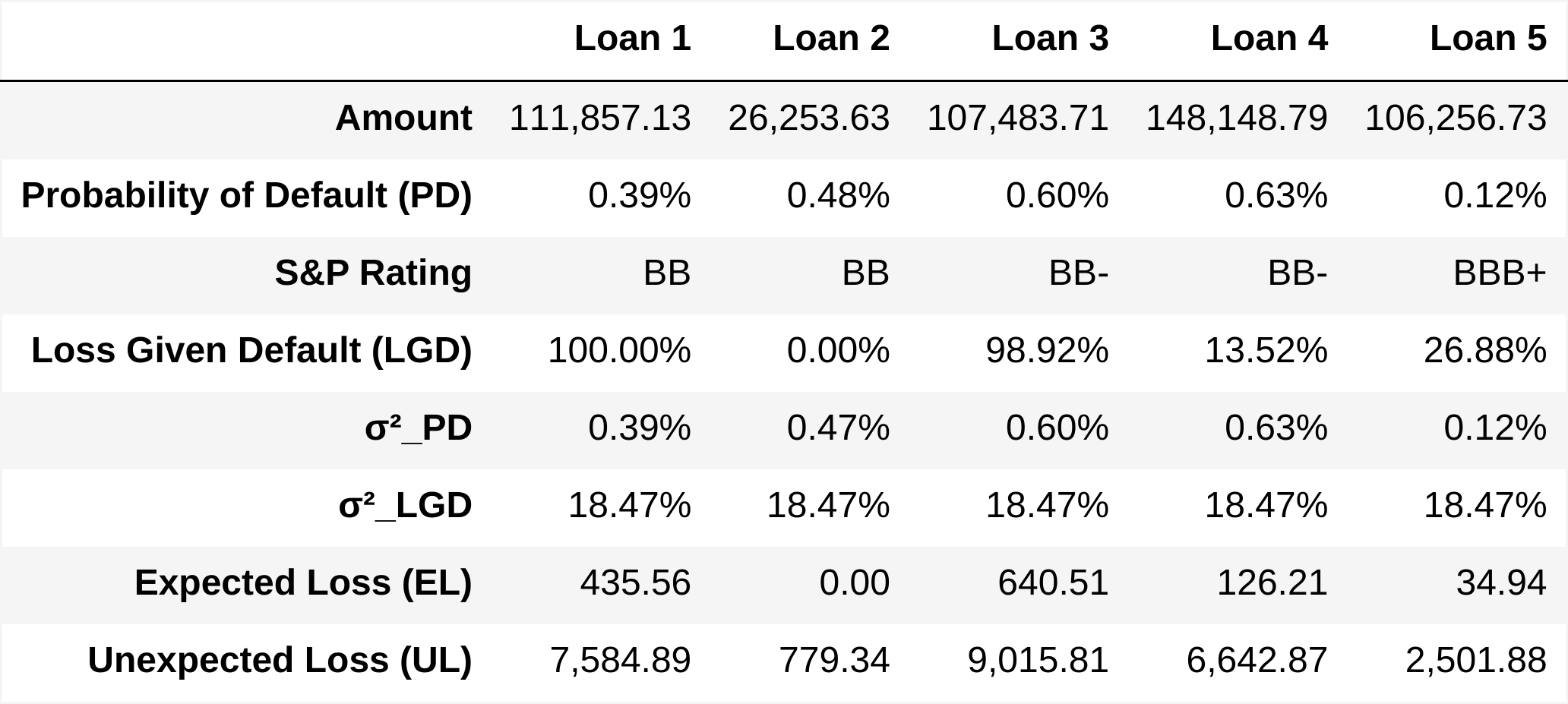
Now, we must combine the above results to find the likely performance of the entire portfolio. Remember when trying to determine the Loss Distribubion, as per formulations above:
expected losses are additive
unexpected losses are not additive
probability of default may be correlated, thereby impacting unexpected loss
We will consider three scenarios:
PD entirely uncorrelated
\(\rho_{ij} = 0 \text{ for all } i,j\)
PD all perfectly correlated
\(\rho_{ij} = 1 \text{ for all } i,j\)
PD correlated
\(.2 < \rho_{ij} < .8 \text{ where }i \neq j\)
Scenarios 1 and 2 can be developed rather easily.
[52]:
p = np.zeros(n)

port_ul1 = port_ul_w_corr(w, ul, p)

p = np.ones(n)
port_ul2 = port_ul_w_corr(w, ul, p)
For Scenario 3, we must prepare a correlation matrix. First we randomly generate the correlation factors.
[53]:
p = np.random.uniform(.2, .8, n)
Then build a 2-D correlation matrix using our hepler function corrs_to_corrmat.
[54]:
print (np.around(corrs_to_corrmat(p), 2))
[[1.   0.38 0.38 0.41 0.78]
 [0.38 1.   0.41 0.78 0.78]
 [0.38 0.41 1.   0.78 0.78]
 [0.41 0.78 0.78 1.   0.78]
 [0.78 0.78 0.78 0.78 1.  ]]
Then, multiply the correlation matrix by the weights and individual expected losses. This is all done inside the helper function port_ul_w_corr.
[55]:
port_ul3 = port_ul_w_corr(w, ul, p)
port_uls = [port_ul1, port_ul2, port_ul3]
This results in the below:
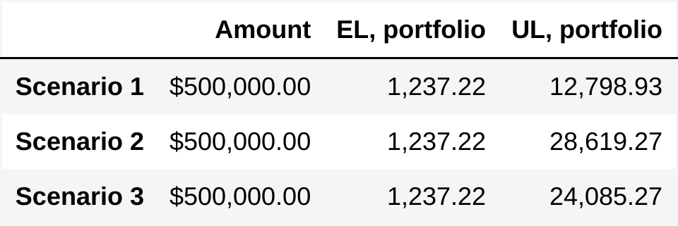
This is below the market average in the US, seen below and found here, but still pretty good for some rough math.
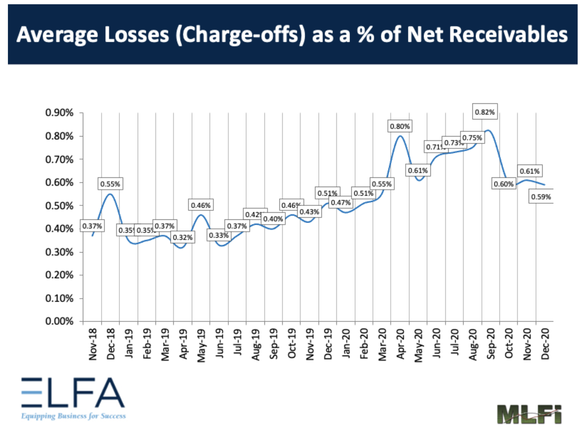
But we should also note that the Unexpected Loss could be 10x-20x more than the Expected Loss in a given year. Should we hold enough capital to absorb the Unexpected Loss? No, we should hold even more than that.
Simulating Losses
To map the Loss Distribution, we must simulate portfolio outcomes based on Loss Model we have constructed.
Goal
Create a sample portfolio from our Loss Model
Generate 50,000 simulations of the portfolio performance in a single year.
The amount of loss in each simulation will be recorded.
A Beta distribution will be fit to the loss record.
Process
Generate
n=20loans totaling $2MM aggregateGenerate PD for each borrower/loan from normal distribution as per here.
Simulate default events
generate
nrandom standard normals, denotedegenerate correlation matrix of defaults across all borrowers for all simulations(values informed by Chapter 7, Appendix B of Ong).
find transformation matrix via Cholesky method
correlated defaults found as
e_primedefaults occur when
e_primeis less than the inverse normal of PD
For each default, generate an LGD based on the distribution used earlier
where the borrower has not defaulted,
LGD = 0%.
[58]:
from scipy.stats import invgauss
from scipy.linalg import eigh, cholesky, svd

# Loan amounts
n = 20
n_samples = 50000

loans_t = 2*10**6
randloans = np.random.uniform(0.1,1,n)
EAD = (randloans / randloans.sum())*loans_t
w = EAD / EAD.sum()

# PD for each borrower/loan.
pd_mu = 0.0044
pd_std = 0.002
p_of_d = np.random.normal(pd_mu, pd_std, n)
p_of_d = np.where(p_of_d<0, 0, p_of_d)
pd_var = bern.var(p_of_d)

# Correlation matrix
e = norm.rvs(0, 1, size=(n, n_samples)) # this creates defaults for ALL borrowers in ALL simulations
p = np.random.uniform(.01, .13, n)
corrmat = corrs_to_corrmat(p)

c = cholesky(corrmat, lower=True)

e_prime = np.dot(c, e).T
pd_inv = np.repeat(norm.ppf(p_of_d), n_samples).reshape(n_samples, n)
If \(e\prime_{i,j} < N^{-1}(PD_{i})\) for any \(i,j\) then borrower \(i\) defaulted in simulation \(j\)
[59]:
in_default = e_prime < pd_inv
print (in_default.shape)
(50000, 20)
in_default is now a boolean array where True means default and False means no default for every borrower (20) in every simulation (50,000).
As a check, we can sum all the defaults and divide by the total number of instances of borrowers (n borrowers X n_samples).
[60]:
default_per = (e_prime < pd_inv).sum() / (n*n_samples)
print (default_per)
0.004452
The process resulted in 0.45% defaults which aligns closely with the expected value of 0.44% mean of the Normal distribution used.
Now, randomly generated LGDs for only those loans that defaulted.
[62]:
# LGD
mean = .4
lgd_std = .4
a, b = beta_params_from_descript(mean, lgd_std**2)
lgds = np.zeros(shape=in_default.shape) # LGDs for all loans start at 0%

i_loss = np.argwhere(in_default)
lgd_rands = beta.rvs(a, b, size=i_loss.shape[0])

# Insert LGDs where there was a default
for i in range(i_loss.shape[0]):
    x, y = i_loss[i]
    lgds[x, y] = lgd_rands[i]
Finally, we multiply the loan amounts by the LGDs to get the loss on every loan in every simulation.
[63]:
losses = np.repeat(EAD, n_samples).reshape(n_samples, n) * lgds

simloss = losses.sum(axis=1)
simloss_gt0 = simloss[simloss>0]

print (simloss.shape[0], simloss_gt0.shape[0])
50000 4180
simloss_gt0 is now an array of simulations where loss was greater than 0. We can see from the above, out of 50,000 simulations, only 4,180 had any defaults. The small size of the portfolio skews the distribution and so simulations with losses of zero will be ignored for distribution fitting.
A few key statistics from the data
Average losses in each year: $3,284.02
Average Percentage Losses: 0.16%
Number of years with 0% loss: 45,820
Average losses in years with loss: $39,282.59
Average Percentage Losses in years with loss: 1.96%
Maximum Loss in any Year: $331,577.44
Now we can fit the distribution and plot it against the simulation.
[66]:
with warnings.catch_warnings():
    warnings.filterwarnings("ignore")

    lnspc = np.linspace(0, simloss_gt0.max(), len(bins))
    params = beta.fit(simloss_gt0)
    ld = beta(*params)
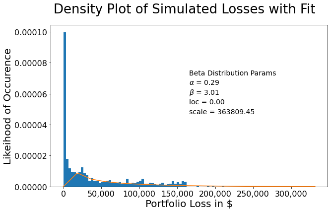
FINALLY, we can find the amount of equity HTS Fico should hold at the 99.95% VAR level of our loss distribution, good enough for a AA credit rating.
[68]:
print (ld.ppf(0.9995))
309417.7141661356
If Fico has a $2MM loan portfolio with the characteristics described here, it should have equity of at least $309,417.71.
Looking closer at the distribution, in the vast majority of cases this amount would protect against solvency, however, it must be noted that in 4 out of the 50,000 simulations, the loss would exceed the equity base and Fico would be in default.